1. Centered Moving Average versus Arithmetic Progression. 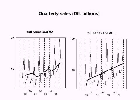In the illustration "Quarterly Sales" a time series (quoted in Appendix A) is depicted, on the left side including a centered moving average (MA), on the right side an "average growth line" (AGL) is added. The series depicts a 7-years stretch (1989 through 1995) of quarterly sales of consumer durables. The terms of the inspected section of the series will be called y1 through y28. At both extremes two terms have been added (y0, y-1, y29, y30) to allow the centered moving average to reach all the terms of the inspected section. Centered moving average: The average value for each group of corresponding quarters, as calculated from the moving average, will be called "unseasonal quarter averages". If these unseasonal quarter averages are subtracted from the quarter averages of the full series we obtain a (preliminary) set of average seasonal components. Average growth line: The average growth line is a straight line through the series' average value (A).                 A = å yi /28 (i = 1, 2, ….., 28) The gradient of this line is the average change ("growth", g) of each term over the preceding term:       g = å (yi -yi-1)/28 = (y28 -y0)/28 (i=1,2,…..,28) The average value for each group of corresponding quarters as calculated from the average growth line coordinates will also be called "unseasonal quarter averages" and they are represented by an arithmetic progression with difference g and average value A:                 A - 1.5g , A - 0.5g , A + 0.5g , A + 1.5 g In general terms the progression can be expressed as:                 A + {i - (p+1)/2}g,        (p = periodicity, i = 1, 2, …, p)                                            (formula 1) Table 1: seasonal components. Full calculation in Appendix A       A = 14741      g = 99 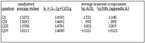Some reflection will make it clear, that unseasonal quarter averages as calculated from the moving average and from the average growth line coordinates should be the same - with the exception that the moving average includes two more terms at the beginning of the series and at the end of the series. But for this exception , moving average and arithmetic progression would render the same seasonal pattern. This will be elaborated below. Which terms figure in a corresponding-quarters-average of a centered moving average? The average for quarters I includes: y1, 1989.I: y-1 + y0 + y1 + y2          y0 + y1 + y2 + y3 four terms centered between y0 and y1 four terms centered between y1 and y2 4 x 2 terms centered at y1 y5, 1990.I: y3 + y4 + y5 + y6         y4 + y5 + y6 + y7 .................... ...................................... y25, 1995.I: 7-years total: y23 + y24 + y25 + y26           y24 + y25 + y26 + y27 ____________________ y-1 + 2 å yi + y27 (i=0, 1, ..., 26) The first-quarters-average is arrived at by dividing the total by (7 x 4 x 2 =) 56. Average Q.I    = (y-1 + 2 å yi + y27) / 56 (i=0, 1, ..., 26) Likewise for the other groups of quarters: Average Q.II   = (y0 + 2 å yi + y28) / 56 (i=1, 2, ..., 27) Average Q.III  = (y1 + 2 å yi + y29) / 56 (i=2, 3, ..., 28) Average Q.IV  = (y2 + 2 å yi + y30) / 56 (i=3, 4, ..., 29) The average value (A) of the inspected section of the series = å yi / 28 (i= 1, 2, …,28). The quarter averages can be rewritten as: Average Q.I    = A - (y28 - y0)/28 - (y27 - y-1)/56 (formula 2) Average Q.II   = A - (y28 - y0)/56 Average Q.III  = A + (y29 - y1)/56 Average Q.IV  = A + (y29 - y1)/28 + (y30 - y2)/56 Note that unseasonal period averages of a centered moving average can be arrived at without first working out the moving average itself. The inside-brackets part of each quarter-average represents growth over the full section of the series, always from a quarter at the beginning of a series to a corresponding quarter at the very end. If unseasonal fluctuations do not distinguish between the periods of the year and if no outliers would occur in the relevant terms, then these growth figures should be more or less the same. This average growth will be called g ', where g ' is variable.                            g ' = (ye - yb)/28 (ye indicates a quarter in the last year of the series, yb a corresponding quarter at the beginning, where e - b = 28). The quarter averages can now be rewritten as: Average Q.I    = A - 1.5g ' Average Q.II   = A - 0.5g ' Average Q.III  = A + 0.5g ' Average Q.IV  = A + 1.5g ' or Average Qi = A + {i - (p+1)/2}g ',       (p = periodicity, i = 1, 2, …, p) This formula is similar to formula 1(unseasonal quarter averages from an average growth line). But here g ' is variable and g ' = (ye - yb)/28 includes the additional terms at the extremes of the relevant section of the time series. What would be the advantage of a variable g '? Above the inconvenience of delay I can only think of reasons to reject variability of g ':

the one characteristic that sets seasonal fluctuations apart from other fluctuations, is that seasonality makes a distinction between periods of the year. By contrast trend/cycle fluctuations have the same average effect on each of the year's periods and so should irregular fluctuations if the series is long enough. The very idea of a moving average is a series with only non-distinguishing fluctuations and that means, ideally, the same average growth between quarter averages. Ironically, variability of this growth g ' is inherent to the moving average procedure and therefore, in my view, contrary to its object. A preliminary seasonal pattern is found by comparing unseasonal quarter averages to the full series' quarter averages. Or, in terms of growth, the differences between the full series' averages minus g 'are dubbed seasonal. Then variation of g ' is reflected in the seasonal pattern while it may have unseasonal causes such as outliers or trend breaks in the extreme terms. And if the cause is a shifting seasonal pattern, the centered moving average may not allocate it in the correct quarter: see formula (2), Average QI = A - (1995.IV - 1988.IV)/28 - (1995.III - 1988.III)/56, for example will lower average QI (incrementing its seasonal component) if QIV and/or QIII 1995 have relatively high values. Also, if g ' is not constant the seasonal pattern will not add up to zero.

As I see it, a constant g, that is the arithmetic progression procedure, has many advantages. It must be noted here, that also a constant g = (y28 - y0)/28 is affected by the same unseasonal causes as under 2., however, this error is consistent for all quarter averages and may be dealt with as will be demonstrated in the next paragraphs. Replacing the moving average by an agl means that no time is lost waiting for the current term to become the center of the MA.